Custom analysis of scRNA-seq data with CytoTRACE 2
Pre-computed Datasets
Results
Explore enrichment of CytoTRACE 2 learned genesets in gold-standard datasets
The Geneset Binary Network (GSBN) architecture allows the CytoTRACE 2 model to learn potency-specific marker sets. Here you can explore the enrichment of top N genes that are positively correlated with the model's prediction on 33 gold-standard datasets. The enrichment scores are calculated with Single sample GSEA (ssGSEA) across training and test cohorts, tissue types, cell types and potency categories.
Explore enrichment of genes in gold-standard datasets
Here, we utilize Single Sample GSEA (ssGSEA) to estimate gene set enrichment scores across various cell types, tissues, and potency categories within 33 gold-standard datasets. These include both training and test datasets employed for model development and validation. You can select one or multiple genes from the dropdown menu to explore their enrichment across dataset cohorts and ground truth potency categories. Check our FAQ section for details on which genes are available to explore.
Download Data
Overview of CytoTRACE 2
Under the Hood
Website features
- Analyze publicly available scRNA-seq datasets pre-analyzed with CytoTRACE 2
- Predict absolute developmental potential in a custom scRNA-seq dataset
- Summarize results by known phenotypes
- Identify predicted stemness- and differentiation-associated genes
Frequently asked questions
- What is CytoTRACE 2?
- Why should I use CytoTRACE 2?
- How does CytoTRACE 2 work?
- What do I need to run CytoTRACE 2?
- Should I normalize the data before running CytoTRACE 2?
- What if my dataset includes rare cell types?
- My data appears to be too large to analyze on the website. What is the file size limit to run CytoTRACE 2 on the website?
- What if I have multiple batches of data? Should I perform any integration?
- Which genes can I explore in the “Explore genes” –> “Custom genes” section?
- Does CytoTRACE 2 work with different platforms, tissues, and species?
- Are there limitations to CytoTRACE 2?
- What are the CytoTRACE 2 potency categories?
- What organism can my data be from?
- I still have so many questions, is there someone I can reach out to for help?
What is CytoTRACE 2?
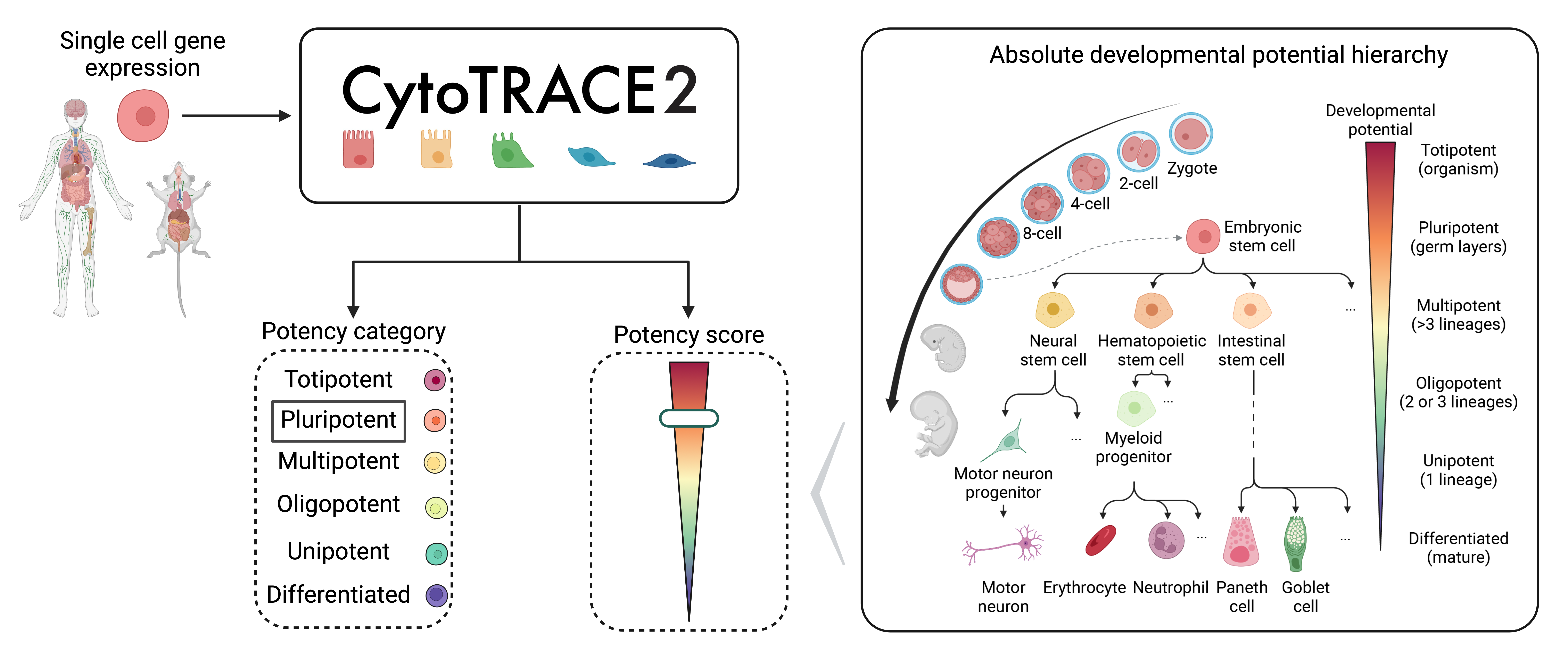
CytoTRACE 2 is a computational method for predicting cellular potency categories and absolute developmental potential from single-cell RNA-sequencing data, across various tissue types, scRNA-seq platforms, and species data. This framework learns multivariate gene expression programs for each potency category and calibrates outputs across the full range of cellular ontogeny, facilitating direct cross-dataset comparison of developmental potential in an absolute space. Underlying this method is a novel, interpretable deep learning framework trained and validated across 34 human and mouse scRNA-seq datasets encompassing 24 tissue types, collectively spanning the developmental spectrum.
More information on why you should use CytoTRACE 2 and how it works is provided below.
Why should I use CytoTRACE 2?
CytoTRACE 2 was developed to predict differentiaton states in scRNA-seq data without any prior information. Some examples where CytoTRACE 2 may be useful, include:
-
Validating differentiation states in tissues with functional evidence of developmental states
-
Assessing absolute developmental potential of cells and comparing these across different datasets
-
Predicting differentiation states in samples where a continuous developmental process is not captured
-
Predicting differentiation states in human tissues where developmental hierarchies are poorly understood
-
Predicting differentiation states in diseased tissues, such as cancer
-
Identifying cells and genes associated with stemness and differentiation
-
Associating cancer cell differentiation states with survival, metastasis, response to therapies, and other clinical outcomes
How does CytoTRACE 2 work?
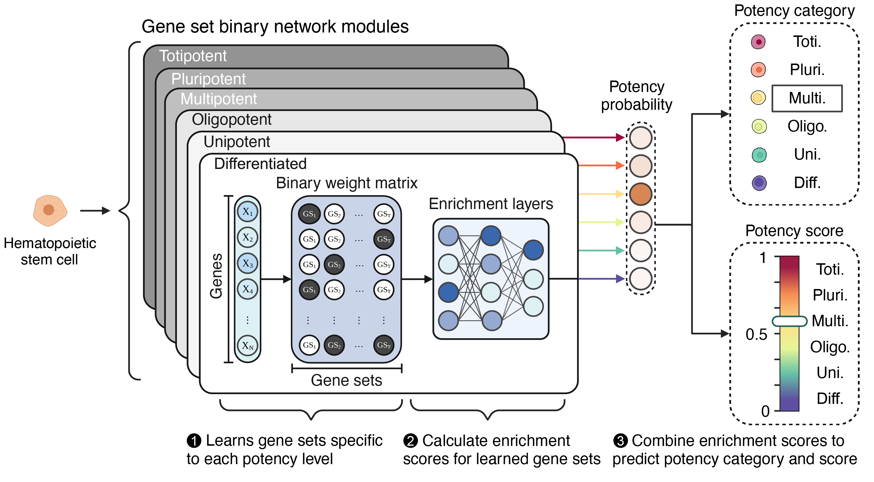
CytoTRACE 2 is designed to assess the absolute developmental potential of cells using a three-step process in its core model architecture. Here’s a simplified breakdown:
-
Preprocessing:
- Ortholog Mapping and Normalization: CytoTRACE 2 first aligns and filters input genes against a unified dictionary of 14,271 mouse/human orthologs, accounting for alias gene names, mapping unused genes to zero. It then transforms the gene expression data into two representations:
- Log2-adjusted CPM/TPM to capture detailed transcriptomic signals.
- Rank space to dampen extreme values and reduce noise. This dual representation provides a robust foundation for subsequent computations.
- Ortholog Mapping and Normalization: CytoTRACE 2 first aligns and filters input genes against a unified dictionary of 14,271 mouse/human orthologs, accounting for alias gene names, mapping unused genes to zero. It then transforms the gene expression data into two representations:
-
Prediction:
- Gene Set Binary Networks: The core model features 19 modules each containing a geneset binary weight matrix for each of the 6 potency categories. Within each module, through numerous matrix operations with the exact weights and parameters learned by training an ensemble model on our training cohort, rank-based and log2 expression-based scores are computed and combined to capture distinct features of gene set activity.
- Integration of Scores: Scores from these operations across potency categories for each member model of the ensemble, across all models, are obtained. For each model both continuous potency scores and softmax output prediction probabilities (to be later mapped to discrete potency categories) are then aggregated to form a consensus prediction of the ensmeble.
-
Postprocessing: The raw predictions of the previous step are then passed through 3 layers of post-processing:
Markov Diffusion Smoothing:
- Utilizes a Markov matrix based on transcriptional similarities to smooth raw potency scores (RPS), resulting in less noisy and more biologically accurate smoothed potency scores (SPS).
Binning Procedure:
- Cells are ranked within their predicted potency categories and uniformly partitioned across the potency spectrum. This ensures that each category spans a specific segment of the range from 0 to 1, refining the smoothed scores (SPSB) to maintain relative order.
Adaptive Nearest Neighbor Smoothing:
- Further refines the binned smooth potency scores (SPSB) for datasets with more than 100 cells by adaptively selecting a neighborhood for each cell, and recalculates each cell’s potency score as a distance-weighted average of its neighbors including itself.
The resulting values are continuous scores ranging from 0 and 1 and discrete labels, representing the predicted absolute developmental potential of cells.
What do I need to run CytoTRACE 2?
All you need to run CytoTRACE 2 is a gene expression matrix generated by single-cell RNA-sequencing, where columns are cells and rows are genes/transcripts. For the website, we require this file to be a text (txt), tab separated value (tsv), or comma separated value (csv) file containing < 5,000 cells. For datasets containing > 5,000 cells, please use the R or Python package implementation. You’ll need to specify your input species (“human” or “mouse”). Phenotype tables are optional, but if included, should be formatted so that the first column contains single cell IDs matching the columns of the gene expression matrix and the second column must contain the labels.
For more details on how to format and upload your data to the website, please refer to the Tutorial page (see sidebar for link).
Should I normalize the data before running CytoTRACE 2?
There is no need to normalize data prior to running CytoTRACE 2, provided there are no missing values and all values are non-negative. The input needs to be raw counts or CPM/TPM data, and should not be log-transformed, as the model employs normalization methods internally.
What if my dataset includes rare cell types?
When analyzing phenotypes expected to have five or fewer cells, we recommend bypassing the KNN smoothing step so that predictions for these rare cells are not forced toward more abundant phenotypes. In practice, you can simply use the preKNN score output (preKNN_CytoTRACE2_Score) instead of the final KNN-smoothed value (CytoTRACE2_Score). This preserves the original predictions for rare cell types while still benefiting from the other postprocessing steps.
My data appears to be too large to analyze on the website. What is the file size limit to run CytoTRACE 2 on the website?
To manage website traffic, we have limited file size uploads to 800 MB. For all datasets greater than 800 MB, please use the R or Python package implementation. You can visit our Github site for detailed instructions on how to install and run these packages.
I have data from multiple batches. Can I still run CytoTRACE 2?
We recommend running CytoTRACE 2 separately over each dataset. While raw predictions are made per cell without regard to the broader dataset, the postprocessing step to refine predictions adjusts predictions using information from other cells in the dataset, and so may be impacted by batch effects. Note that CytoTRACE 2 outputs, except for Relative Order, are calibrated to be comparable across datasets without further adjustment. Therefore, no integration is recommended over the predictions either. As for Relative Order, it should not be compared across different runs, as it is based on the ranking and scaling of CytoTRACE2 Scores within the context of the specific input dataset.
Which genes can I explore in the “Explore genes” –> “Custom genes” section?
For this section utilize Single Sample GSEA (ssGSEA) to estimate gene set enrichment scores across various cell types, tissues, and potency categories within our 34 gold-standard datasets. These include both training and test datasets employed for model development and validation.You can select one or multiple genes from the dropdown menu to explore their enrichment across dataset cohorts and ground truth potency categories. Of note, the genes currently available for exploration are limited to the feature space of CytoTRACE 2, which is comprised of 14,271 total genes, including mouse gene symbols and human gene symbols mapped to mouse orthologs. Accordingly, all queries should use mouse gene symbols. For a list of supported gene symbols, download here.
Does CytoTRACE 2 work with different platforms, tissues, and species?
Although there are some caveats to note (see section ‘Are there limitations to CytoTRACE 2?’ below), CytoTRACE 2 can be applied to scRNA-seq data from any platform, tissue, and species. We show in our original manuscript (Kang et al., 2022) that CytoTRACE 2 is robust to variation in dataset characteristics. Just to note, CytoTRACE 2 was developed over mouse and human data, so datasets supplied to the website should have human or mouse gene names, following HGNC and MGI gene naming conventions.
Are there limitations to CytoTRACE 2?
There are some situations where direct application of CytoTRACE 2 to the dataset would be suboptimal. These include:
Dependence on Feature Overlap with Model Features: CytoTRACE 2’s performance is closely tied to the overlap between the features in the input data and those used by the model. If the overlap in gene features is less than 10,000 genes, the model may show poorer performance, due to not observing the needed level of signal for accurate predictions.
Sensitivity to Low UMI/Gene Counts: Although generally insensitive to variation in gene/UMI counts per cell, CytoTRACE 2 requires further optimization for cells that have exceedingly low gene expression levels, particularly those with fewer than 500 genes expressed per cell, as its performance can become less reliable in these cases. For best results, a minimum gene count of 500-1000 per cell is recommended.
Limitation in Species Generalization: While CytoTRACE 2 is designed for human and mouse data, you can attempt to map gene names from other species to mouse orthologs to utilize the model. However, this approach is experimental and does not guarantee reliable performance without further testing and optimization.
Verification of Predictions: Although the differentiation states and molecular signatures predicted by CytoTRACE 2 are biologically aware and promising, they are preliminary and intended to generate hypotheses. These predictions need to be independently confirmed and functionally validated in future studies.
What are the CytoTRACE 2 potency categories?
CytoTRACE 2 classifies cells into six potency categories:
- Totipotent: Stem cells capable of generating an entire multicellular organism
- Pluripotent: Stem cells with the capacity to differentiate into all adult cell types
- Multipotent: Lineage-restricted multipotent cells capable of producing >3 downstream cell types
- Oligopotent: Lineage-restricted immature cells capable of producing 2-3 downstream cell types
- Unipotent: Lineage-restricted immature cells capable of producing a single downstream cell type
- Differentiated: Mature cells, including cells with no developmental potential
I still have so many questions, is there someone I can reach out to for help?
If you have further questions, please email us at cytotrace2team@gmail.com.
If you have any questions, comments, or concerns regarding CytoTRACE 2, please feel free to send us an email at cytotrace2@gmail.com
Aaron Newman

Minji Kang

Erin L. Brown

Gunsagar Gulati

Jose Juan Almagro Armenteros

Rachel Gleyzer

Susie Avagyan

Wubing Zhang

Brief overview
34 human and mouse scRNA-seq datasets encompassing 24 tissue types were analyzed with CytoTRACE 2.
*Please follow the instructions on the tabs above to analyze pre-computed datasets*.
Load pre-computed datasets
- Navigate to the Run CytoTRACE 2 tab on the website.
- Click on the bar on the top right side of the page under Pre-computed Datasets.
You should now see a drop-down menu listing the datasets that have already been analyzed by CytoTRACE 2. Each dataset is named by biological theme and scRNA-seq platform (e.g. Pancreas (10x)), as shown below:

Once you have selected a dataset to analyze. Click Show results as displayed below.

After viewing results for the selected dataset, in case you want to explore another dataset or upload your custom dataset, click Restart run button at the top right corner to be redirected to the landing page.

To download any of the underlying data, refer to the "Downloads" tab on the left-side panel.
Analyze results I: Low-dimensional visualization
- A useful way to analyze scRNA-seq data is by visualizing a low-dimensional embedding of the data
- We provide an option to visualize your data with Uniform Manifold Approximation and Projection (UMAP) embeddings, which can be colored by
- CytoTRACE 2 values
- CytoTRACE 2 Score - Predicted absolute cellular potency score (continuous). Possible values are real numbers ranging from 0 (differentiated) to 1 (totipotent).
- CytoTRACE 2 Potency - Predicted cellular potency category (discrete). Possible values are Differentiated, Unipotent, Oligopotent, Multipotent, Pluripotent, and Totipotent.
- CytoTRACE 2 Relative Order - Predicted relative order of the cell, based on the absolute predicted potency scores, normalized to the range [0,1] (0 being most differentiated, 1 being least differentiated).


- CytoTRACE 2 values
- Phenotypes (if provided)

- Log-normalized expression of a specified gene of interest (type gene name in the text box)
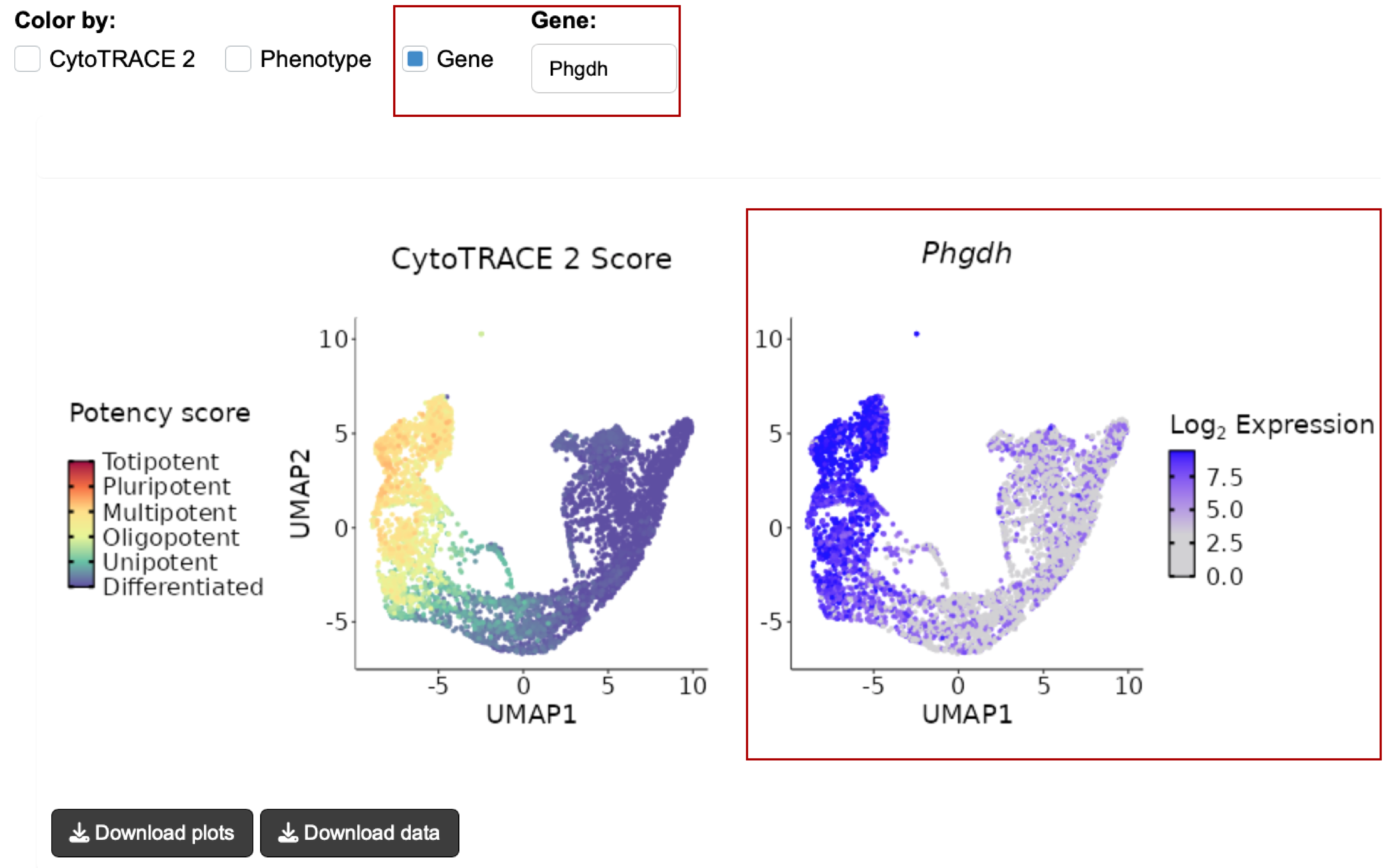
- Plots can be downloaded by clicking the Download plot(s) button on the bottom left.
- Underlying data for the plots (UMAP embeddings, CytoTRACE 2 Scores and specified gene expression data) can be downloaded by clicking the Download data button on the bottom left.
Analyze results II: CytoTRACE 2 by phenotype
- If phenotype labels are available for each single cell, we can summarize the median and distribution of CytoTRACE 2 values per phenotype using boxplots. Boxes are ordered based on the median score of each group.
- The boxplot can be downloaded by clicking the Download plot button on the bottom left.

Analyze results III: Genes associated with CytoTRACE 2
- Genes associated with stemness and differentiation can be predicted based on their correlation with CytoTRACE 2 Score (absolute)
- The following barplot shows the top 10 (less differentiated; red) and bottom 10 (most differentiated; blue) genes in this dataset based on their correlation with CytoTRACE 2
- The barplot can be downloaded by clicking the Download plot button in the bottom left.
- The correlation of every provided gene with CytoTRACE 2 Score can also be downloaded by clicking the Download gene correlations button in the bottom left.

Additionally,
- When selecting Gene from the Color by options, you will also see a boxplot which shows the log-normalized expression of a specified gene against CytoTRACE 2 predicted potency categories.
- The boxplot can be downloaded by clicking the Download plot button in the bottom left.

Brief overview
In this tutorial, we provide instructions to analyze a custom single-cell RNA-sequencing (scRNA-seq) dataset. Users have the option to provide phenotype labels, if available. For the analysis of large datasets (e.g. >5,000 cells), we request users to run the R or Python impementation of CytoTRACE 2.
*Please follow the instructions on the tabs above to analyze a custom scRNA-seq dataset*.
Data format
To make sure the tool runs without issues, please follow the guidlines below on how to prepare your input data:
Gene expression table (required)
CytoTRACE 2 takes as input a scRNA-seq gene expression table with the following formatting requirements:
- The matrix must be genes (rows) by cells (columns). The first row must contain the single cell IDs and the first column must contain the gene names.
- The data must be delimited by either commas, tabs, spaces, or semicolons.
- The data needs to contain either human or mouse genes as its features (adhereing to HUGO and MGI nomenclatures for human and mouse genes accordingly)
- It has to include either non-normalized raw counts or CPM/TPM normalized expression values, and should not be log-transformed.
- Please DO NOT pre-filter the genes in the expression matrix.
Phenotype table (optional)
Users can choose to provide phenotype labels corresponding to the single cell IDs in the gene expression matrix. Please prepare the phenotype table in the following format:
- The table should contain at least two columns, where column 1 contains the single cell IDs corresponding to the columns of the scRNA-seq matrix and column 2 contains the corresponding phenotype labels. Any additional columns will be ignored.
- The table should contain a header.
- The table must be delimited by either commas, tabs, spaces, or semicolons.
- To make sure the phenotype labels are properly placed on top of visualizations and are not cut-out, you can try to abbreviate the labels and keep under 25 character limit.
Download vignette datasets
We provide two small vignette datasets you can download below and use to test-drive CytoTRACE 2 before preparing your own files: Each download is a .zip file containing:
*_expression.txt— a genes × cells matrix (rows = genes, columns = cells)*_annotation.txt— a two-column phenotype table (first column = cell IDs that match the expression columns, second column = cell types)
Run CytoTRACE 2
Upload your gene expression table (required)
- After formatting your gene expression table as instructed in the Prepare data tab:
- Navigate to the Run CytoTRACE 2 tab
- Click the Browse button to upload your data
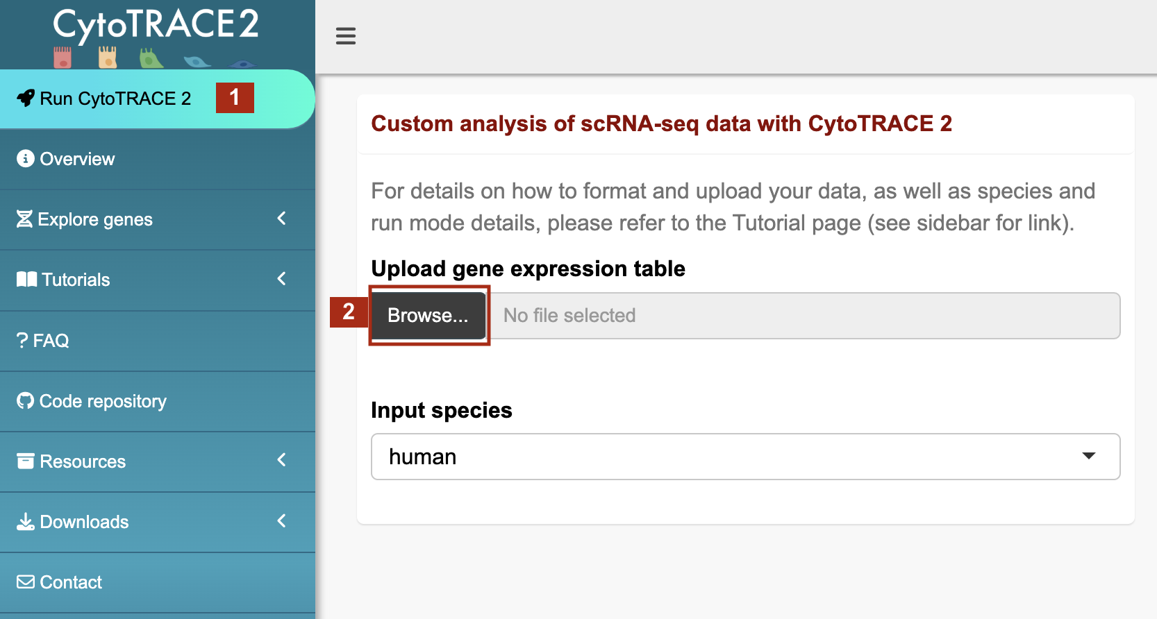
3. Choose the appropriate species for your input (human or mouse)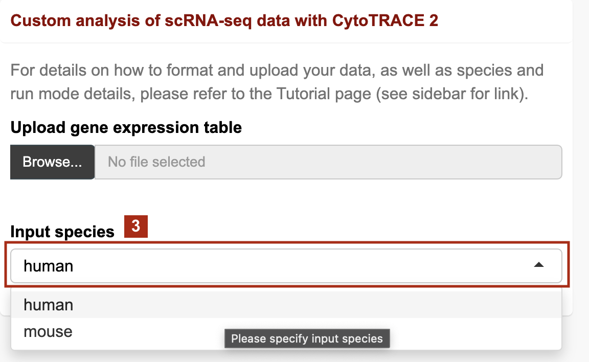
4. If you have prepared a phenotype file as well, upload here: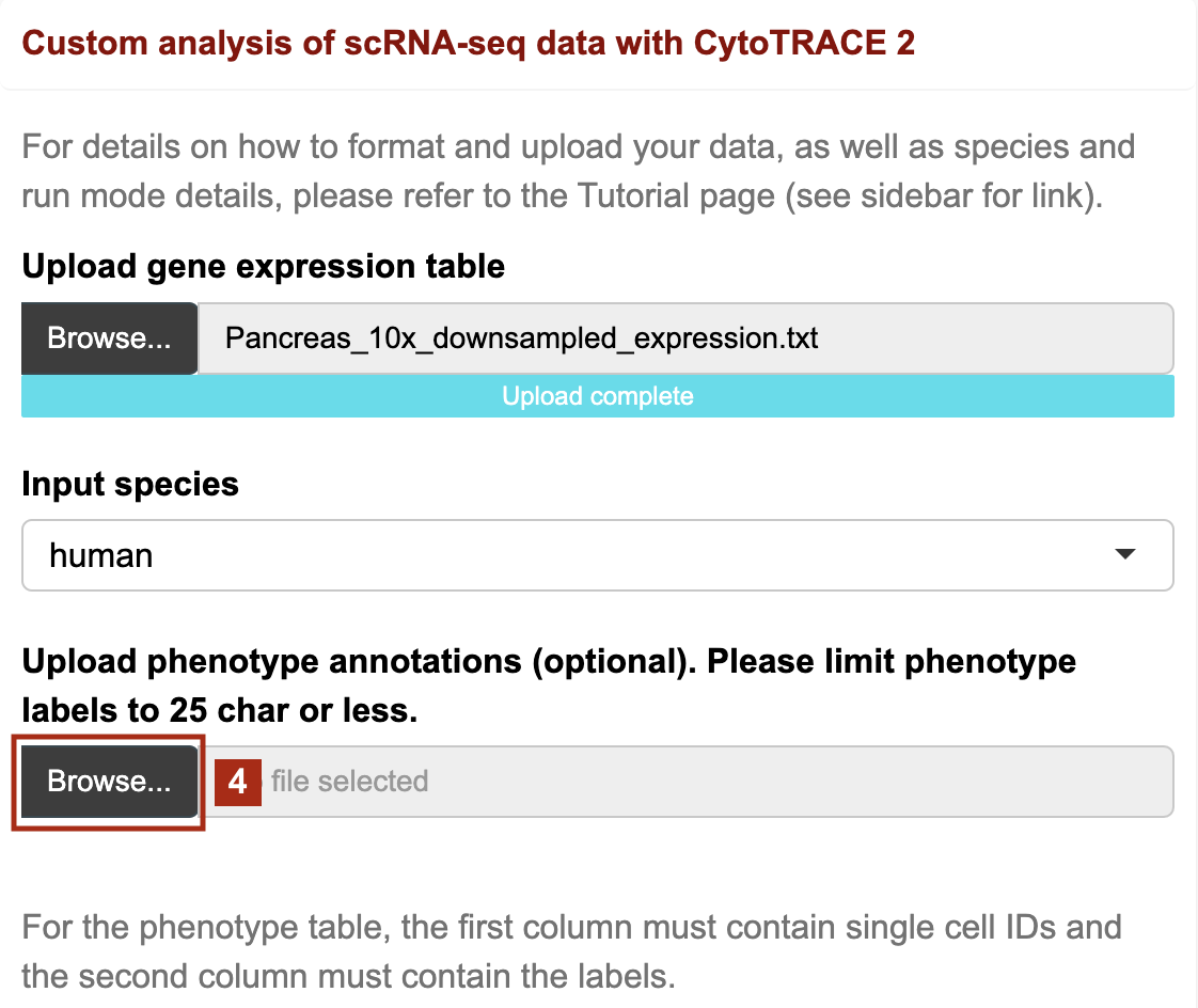
Run CytoTRACE 2
After uploading all your files and selecting input options, click Run CytoTRACE 2. Running CytoTRACE 2 may take some time with large datasets. Once the analysis is complete, you will be directed to a another page with the results of your run. These are detailed in the next three tabs.

Analyze results I: Low-dimensional visualization
- A useful way to analyze scRNA-seq data is by visualizing a low-dimensional embedding of the data
- We provide an option to visualize your data with Uniform Manifold Approximation and Projection (UMAP) embeddings, which can be colored by
- CytoTRACE 2 values
- CytoTRACE 2 Score - Predicted absolute cellular potency score (continuous). Possible values are real numbers ranging from 0 (differentiated) to 1 (totipotent).
- CytoTRACE 2 Potency - Predicted cellular potency category (discrete). Possible values are Differentiated, Unipotent, Oligopotent, Multipotent, Pluripotent, and Totipotent.
- CytoTRACE 2 Relative Order - Predicted relative order of the cell, based on the absolute predicted potency scores, normalized to the range [0,1] (0 being most differentiated, 1 being least differentiated).
- CytoTRACE 2 values
- Phenotypes (if provided)
- Log-normalized expression of a specified gene of interest (type gene name in the text box)
- Plots can be downloaded by clicking the Download plot(s) button on the bottom left.
- Underlying data for the plots (UMAP embeddings, CytoTRACE 2 Scores and specified gene expression data) can be downloaded by clicking the Download data button on the bottom left.
Analyze results II: CytoTRACE 2 by phenotype
- If phenotype labels are available for each single cell, we can summarize the median and distribution of CytoTRACE 2 values per phenotype using boxplots. Boxes are ordered based on the median score of each group.
- The boxplot can be downloaded by clicking the Download plot button on the bottom left.
Analyze results III: Genes associated with CytoTRACE 2
- Genes associated with stemness and differentiation can be predicted based on their correlation with CytoTRACE 2 Score (absolute)
- The following barplot shows the top 10 (less differentiated; red) and bottom 10 (most differentiated; blue) genes in this dataset based on their correlation with CytoTRACE 2
- The barplot can be downloaded by clicking the Download plot button in the bottom left.
- The correlation of every provided gene with CytoTRACE 2 Score can also be downloaded by clicking the Download gene correlations button in the bottom left.
Additionally,
- When selecting Gene from the Color by options, you will also see a boxplot which shows the log-normalized expression of a specified gene against CytoTRACE 2 predicted potency categories.
- The boxplot can be downloaded by clicking the Download plot button in the bottom left.
Development of the CytoTRACE 2 package
The CytoTRACE 2 prediction algorithm is available as both an R package and a Python package, enabling you to download and run it locally. For comprehensive resources including the package scripts, detailed documentation, vignettes, and input examples, please visit our GitHub repository.
Inventory of ground truth datasets
This collection of datasets comprises publicly available single-cell RNA sequencing (scRNA-seq) data with cell annotations, including phenotype, ground truth potency labels, and absolute and granular developmental orderings used for training and testing the CytoTRACE 2 model. To download, click on any dataset, then click on the 'Download dataset' button below the table. We also provide an option to download all datasets in a compressed file by each cohort.
Download datasetDownload all (by cohort)
Extended annotations for large dataset cohorts
This section provides full, cell-level annotation files for several large cohorts used in our study, which were downsampled for the analysis in the paper for computational feasibility. Details of the downsampling are as follows:
- Tabula Muris: downsampled to 30 cells per phenotype within each tissue–platform pair.
- Tabula Sapiens: downsampled to 100 cells per phenotype within each tissue–platform pair.
- Immune cell atlas (10x), Human breast 1 (10x), and Human breast 2 (10x): downsampled to 100 cells per phenotype.
License agreement
STANFORD NON-COMMERCIAL SOFTWARE LICENSE AGREEMENT
- The Board of Trustees of the Leland Stanford Junior University (“Stanford”) provides CytoTRACE 2 software and code (“Service”) free of charge for non-commercial use only. Use of the Service by any commercial entity for any purpose, including research, is prohibited.
- By using the Service, you agree to be bound by the terms of this Agreement. Please read it carefully.
- You agree not to use the Service for commercial advantage, or in the course of for-profit activities. You agree not to use the Service on behalf of any organization that is not a non-profit organization. Commercial entities wishing to use this Service should contact Stanford University’s Office of Technology Licensing and reference docket S24-057.
- THE SERVICE IS OFFERED “AS IS”, AND, TO THE EXTENT PERMITTED BY LAW, STANFORD MAKES NO REPRESENTATIONS AND EXTENDS NO WARRANTIES OF ANY KIND, EITHER EXPRESS OR IMPLIED. STANFORD SHALL NOT BE LIABLE FOR ANY CLAIMS OR DAMAGES WITH RESPECT TO ANY LOSS OR OTHER CLAIM BY YOU OR ANY THIRD PARTY ON ACCOUNT OF, OR ARISING FROM THE USE OF THE SERVICE. YOU HEREBY AGREE TO DEFEND AND INDEMNIFY STANFORD, ITS TRUSTEES, EMPLOYEES, OFFICERS, STUDENTS, AGENTS, FACULTY, REPRESENTATIVES, AND VOLUNTEERS (“STANFORD INDEMNITIES”) FROM ANY LOSS OR CLAIM ASSERTED AGAINST STANFORD INDEMNITIES ARISING FROM YOUR USE OF THE SERVICE.
- All rights not expressly granted to you in this Agreement are reserved and retained by Stanford or its licensors or content providers. This Agreement provides no license under any patent.
- You agree that this Agreement and any dispute arising under it is governed by the laws of the State of California, United States of America, applicable to agreements negotiated, executed, and performed within California.
- Subject to your compliance with the terms and conditions set forth in this Agreement, Stanford grants you a revocable, non-exclusive, non-transferable right to access and make use of the Service.
Download license